Basics of Quantification & digital PCR Assay Design

Digital PCR (dPCR) provides highly precise quantification of nucleic acids. Its core principles involve partitioning a sample into thousands of droplets, each acting as an individual reaction chamber. The dynamic amounts of positive and negative droplets as well as the average volume of the droplets are then used to predict the average target nucleic acid copy number using the Poisson distribution as the model that describes rare event detection.

For example, let’s imagine our 20 µL sample contains 6 copies of target DNA (gene X) that we want to detect and quantify. If we disperse our sample into a large number of small partitions, assuming the partitioning is random and independent, this process can be described using a Poisson distribution (see the image below).

It does not really matter where the 6 copies of our target gene X end up—whether they all end up in different partitions, all in the same partition, or something in between. The probability of each of these scenarios can be denoted as p. Let’s assume that we have 20,000 partitions. Since we only have 6 molecules, it makes sense that they are most likely to end up in different partitions, given the large number of partitions (20 000).

Of course, it is theoretically possible that all 6 molecules will end up in the same partition. However, considering the overwhelming number of partitions compared to the number of gene X molecules, and the fact that the molecules are dispersed in a 20 µL solution (making them likely far apart), this outcome is extremely unlikely.

If we repeatedly partitioned our 6-molecule sample many times (n repetitions), we could plot the probabilities (“Prob”) of observing partitions containing 0 gene X molecules (“Copies”), 1 gene X molecule, 2 gene X molecules, 3, 4, 5, and 6. As expected, most of our droplets after partitioning would be empty. The second most common event would be droplets containing a single target gene X molecule. Much less frequently, we would observe droplets containing more than one gene X molecule.

This distribution describes the probabilities (or frequencies) of discrete events—essentially, the likelihood of observing negative droplets, single-copy droplets, two-copy droplets, and so forth.

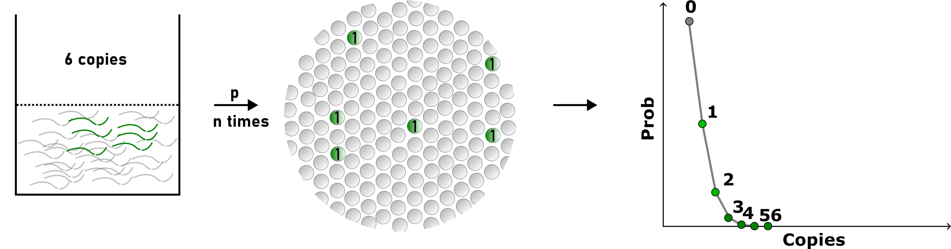
An illustration on how sample partitioning and Poisson distribution-based, average copy number per partition determination is carried out (theoretical example)

Okay, so what of it (you might ask yourself)? Well, what we have just described is a Poisson distribution, and we can calculate it’s single parameter lambda, which will be our average copy number per droplet (CPD), using the following simplified formula:

𝐶𝑃𝐷=−ln⁡(𝑁_𝑛𝑒𝑔/𝑁_𝑡𝑜𝑡𝑎𝑙 )/𝑉_𝑑𝑟𝑜𝑝𝑙𝑒𝑡 (0.0003 copies/ul in our example case)

Where:

N_neg - Number of negative droplets

N_total - Number of total droplets

V_droplet - Average droplet volume

Using the ratio of the number of negative partitions to all partitions, divided by the average volume of the partition we can easily find the CPD. If we want to know the total number of copies in our initial sample we just multiply our CPD by the total number of partitions observed in that sample (for ddPCR that’s around 20 000):

𝐶𝑜𝑝𝑖𝑒𝑠/(20 𝑢𝑙)=𝐶𝑃𝐷×𝑁_𝑡𝑜𝑡𝑎𝑙 (≈20 000) (0.00003 x 20 ul = 6 copies)

Relationship Between the Limit of Detection and Interrogated Molecules, the Rule of Three

The level of limit of detection (LOD; of an assay) and the number of interrogated genome equivalents are deeply intertwined parameters. Since in practice (and according to Poisson statistics) it has been observed that in order to detect 1 positive event out of 1 000 (i.e. achieve an LOD of 0.001 or 0.1%), approximately three times more genome equivalents must be screened (in this example, ~3 000 genome equivalents must be interrogated). In ddPCR, because DNA molecules are distributed into droplets according to Poisson statistics, this requires generating a larger number of droplets depending on the mean occupancy. We can therefore describe the relationship between LOD and the number of interrogated molecules as:

p = 3 / N

Where:

p - sensitivity

N - number of molecules interrogated

Thus, to detect a rare mutation present at a 0.1% allele fraction with 95% confidence, approximately 3,000 genome equivalents must be interrogated.

In practise, a common heuristic of determining whether a sample is positive or not is to first determine the FPR (False positive rate) by running NTCs (i.e., Non-template control samples), determining the number of positive droplets and then multiplying the number of positive droplets obtained in the NTC samples by 3. Samples containing at least 3 times higher number positive droplets than the FPR are then very likely to be positive.

The Most Common ddPCR Assay Types

Copy number determination. ddPCR allows for the accurate and absolute quantification of gene (target) copies. One can even contrast and compare the measurements to a reference gene (which can be run in another channel) in order to see any discrepancies in copy number variations, such as gene (target) duplications. This simultaneous quantification of multiple targets within the same reaction is achieved by using sequence-specific hydrolysis probes labelled with different fluorescent dyes. Copy number determination methods are particularly useful in applications like quantifying plasmid copies in gene therapy, multiple (and simultaneous) pathogen detection or assessing gene amplification in cancers.

Mutation detection. ddPCR is particularly advantageous because it can discriminate between wild-type and mutant alleles with exceptional sensitivity. By designing assays that target specific mutations, one can quantify the fraction of mutant DNA within a heterogeneous sample. This is especially valuable in personalized medicine approaches such as cancer diagnostics, where detecting low-abundance mutations can inform treatment decisions.

See the image below for a simple summary.

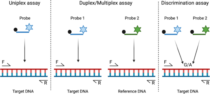source: Baltrusis et al., 2023, Figure 2