Gene Expression Assay Setup

The following short guide is based on the publication by S.C. Taylor et al., 2019. The original article has a lot of great tips and insight, especially for qPCR beginners. I highly recommend reading through it at least once. If you’re not sure how to design a primer pair for your target, you can always refer to the section on Primer and Probe Design.

The First Experiments

Let’s say you’ve placed an order and received a new primer pair and your goal is to validate and test these primers in a qPCR reaction using your existing batch of RNA/cDNA samples (refer to MIQE guidelines by Bustin et al., 2009, section “Nucleic Acid Extraction” in Table 1 for the minimal information required on the extracted samples and their quality). Here’s some key steps that you should consider:

I. Pooling your samples and diluting: Since all your different samples could potentially to have varying amounts of inhibitors (due to e.g. different extraction time-points, different biological conditions, etc.), pool all (or some) of your existing samples to make the most representative pan-sample for the subsequent downstream qPCR analyses. Optionally you could dilute that pool 1:10 or 1:20.

II. First experiment - Thermal Gradient Optimization: The very first experiment you should consider running is the optimization of your qPCR primer pair (& probe if applicable) via an annealing temperature gradient (e.g. 50-60/55-65 degrees). For SYBR green applications, make sure you insert a melt curve analysis at the end of your amplification protocol (that is, after the 35-40 cycles of the annealing temperature experiment, insert a final, e.g. 55 to 95 degrees, at 0.5 degrees increment, step). The reason behind the inclusion of the melt curve analysis step is that, at the end of this compound experiment, you will not only find out the optimal annealing temperature, but also the specificity of your primer pair (and hopefully no off-target amplification). If running probe(s) - melt curve analysis is not possible. However, to remedy this, make sure to visualize your qPCR product band(s) on an agarose gel instead. If only a single band is present - this means your qPCR primer and probe pair are specifically amplifying the target of your choice.

By conducting this experiment you will satisfy the points 1 & 2 in the MIQE guidelines, “qPCR validation” in Table 1.

III. Second experiment - Standard Curve and Efficiency Testing: The second experiment encompasses making a dilution series of your pooled sample and running these dilutions in qPCR at the optimal annealing temperature (as determined in the first experiment). The magnitude of the dilution depends solely on the initial Cq value you obtained for the curve with the optimal annealing temperature in the first experiment. Depending on that initial Cq value you got, you should make a serial dilution of your pooled sample at either 1:2 (Cq is 23-), 1:4 (Cq is 16-23) or 1:8 (Cq is 10-16) ratios of sample:sample+water.

EXAMPLE: Let’s say in your first experiment you determined the optimal annealing temperature to be Ta=55 degrees, because out all the different annealing temperatures, the reaction at 55 degrees produced the sigmoidal curve that has the lowest Cq value (=18). Therefore, you should make serial dilutions of your pan-sample at 1:4 ratios of sample:sample+water.

In addition to running the serial dilutions of your pooled sample, make sure to include the necessary controls and replicates (at least 2 or 3 technical replicates) in the experiment. At the very least an NTC should be run in parallel with all your experiments. Since qPCR and digital PCR share a lot of similar control types, i recommended checking out the section on Control Sample Types in ddPCR and picking the most relevant controls for your experiments.

After having run the second experiment comes the most critical part in the primer validation step - the determination of the reaction efficiency. Typically, your qPCR software plots the standard curves and provides the most important measurements (such as r-squared value, a.k.a. linearity, slope, and efficiency) for you. Your end-goal for this experiment to obtain the reaction efficiency somewhere between 90%-110%. Reaction efficiencies below 90% indicate sub-optimal amplification and likely mean you have to redesign your primers, whereas efficiencies above 110% point to some sort of polymerase inhibition (and thus improved amplification at higher dilutions), which should be addressed by reviewing the sample preparation process and eliminating the source of potential inhibitors.

Once you’ve established a standard curve using your pooled sample (data from the second experiment), ensure that your subsequent RNA/cDNA sample Cq values land in or ideally around the middle of the linear dynamic range of your assay (by diluting or running higher volumes of your samples).

By conducting the second experiment (+ including relevant controls) you will have enough data to satisfy the points 3-11 in the MIQE guidelines, “qPCR validation” in Table 1.

Controls

I can’t stress the importance of running adequate controls for your experiments. Have a look at the Control Sample Types in ddPCR to get an idea of the type of controls you would likely need in your qPCR experiments. For example, you might consider running:

Negative template control(s), in order to ensure there’s no reagent contamination with the amplicon or that your primer pair does not produce any false positive (nonspecific) signal in the absence of the template.

no-RT control(s), to monitor for the presence of gDNA contamination, which can yield a false positive signal in your qPCR experiments. If gDNA is indeed present and detected, make sure to treat your RNA samples with the DNAse enzyme(s) to remove it prior to the reverse transcription step.

Positive control(s), to make sure that all your reagents are functional. If for some reason your qPCR reactions and the subsequent Cq values look strange, a positive control - typically a custom gBlock ssDNA or a plasmid with a cloned amplicon - can help you figure out if there are issues with your reagents.

Although typically not referred to as a control - replicates play a crucial part in running your qPCR experiments. Since qPCR tends to be rather variable (compared to e.g. digital PCR), you might want to include 2 or 3 replicates of each sample, in order to evaluate the degree of Cq value variation, most often expressed in terms of %CV (coefficient of variation). Keep in mind that running the same sample in multiple qPCR reactions (under the same conditions) is referred to as running technical replicates. Whereas testing different biological samples (for example, different batches of the same type or species of cells/tissue/organism etc.) that have been processed and run under the same conditions is referred to as running biological replicates. Biological replicates, unlike technical replicates, are essentially used to evaluate if a similar response is elicited (e.g. gene expression profiles for your target) in different biological systems (of the same type or species).

Reference genes

In order to understand what happens to your gene target at different biological conditions (such as before and after treatment with a drug), you would typically want to normalize your gene expression data (i.e. Cq values) to a stably expressed, house-keeping gene. This will in turn help you identify any potential changes in expression (down-regulation/up-regulation) due to the change in the biological circumstances. Multiple companies sell house-keeping gene assays that can be readily used to evaluate the stability of those reference gene in your samples. It might also be useful to look through the literature for primer pairs used in gene expression experiments (with your model organism) or even talk to your colleagues. Whichever strategy you choose - it’s important you test the stability of the reference genes in YOUR samples in different biological conditions (e.g. pre & post exposure to specific drugs you are working with), since some reference genes might actually not be stable in your samples, especially after exposure to treatment. Examples of the software that can help you with reference gene stability evaluations is GeNorm and Bio-Rad’s Reference Gene Selector Tool in CFX Maestro.

Alternative Approach

If at any point the experimental data proves to be unstable and thus unusable (for example, due to low reaction efficiency, low consistency & high variability), consider switching to digital PCR. Digital PCR is typically less susceptible to inhibitors, requires no standard curves aand, more importantly, is a much more precise technique - thanks to the partitioning step prior to PCR.

For a summary workflow, refer to the diagram below. 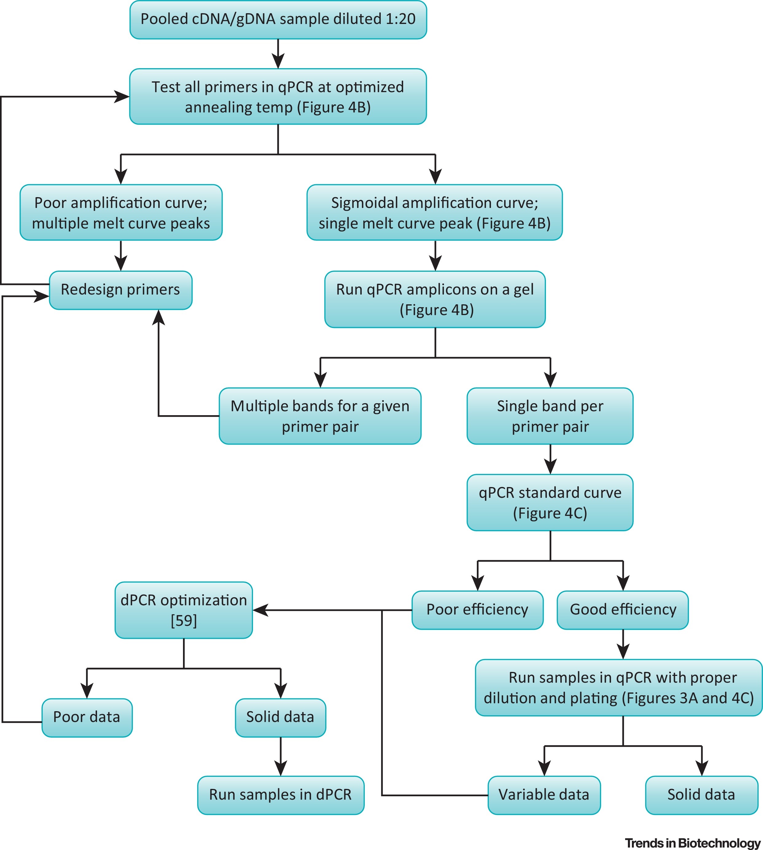source: S.C. Taylor et al., 2019 Figure 6